Getting Started

Example 101

This is an example which solves a cube with a Saint Venant-Kirchhoff (SVK) material for the case of uniaxial loading. In the first step, we init a model.

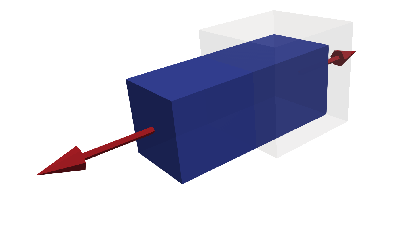
Deformed unit-cube with normal forces and surface 1.

import cubrium

MDL = cubrium.init()

Constitution

In the second part, we have to define the constitutive law. We can either use one of cubrium’s models or use our own umat (user material). This time we’re using our own umat function for a simple Saint Venant-Kirchhoff material.

(1)\[\boldsymbol{S} = 2\mu\ \boldsymbol{E} + \gamma\ \mathrm{tr}(\boldsymbol{E}) \ \boldsymbol{1}\]

import numpy as np

def umat_svk(F, parameters):
    """(U)ser (MAT)erial Function.
    Returns First Piola-Kirchhoff stress tensor for a given
    deformation gradient tensor with a list of material parameters."""

    # expand list of material parameters
    mu, K = parameters[:2]
    gamma = K - 2 / 3 * mu

    C = F.T @ F
    E = 1 / 2 * (C - np.eye(3))

    S = 2 * mu * E + gamma * np.trace(E) * np.eye(3)

    return F @ S

Now we have to link our umat to the cubrium model definition and specify material parameters.

MDL.GLO.constitution.umat       = umat_svk
MDL.GLO.constitution.parameters = [1.0, 5000.0]

Loadcase (Kinematics and Kinetics)

A loadcase is defined with exactly 9 equations for the unsymmetric or 6 equations for the full-symmetric case. This contains either kinematic or kinetic types of equations. For the case of uniaxial loading we are building this loadcase for ourselfes. We apply an external normal force 1 and set all external shear forces and normal forces 2 and 3 to zero. A symmetric solution is enforced (no rigid body rotation is allowed). The load-proportionaly-factor is applied to the normal forces (lpftype=0). Finally we specify a title for the loadcase. This will later effect the output filenames.

def uniaxial(MDL):
    MDL.EXT.force.normal[0] = 1
    MDL.EXT.force.normal[1] = 0
    MDL.EXT.force.normal[2] = 0

    MDL.EXT.force.shear[0, 1] = 0
    MDL.EXT.force.shear[1, 2] = 0
    MDL.EXT.force.shear[0, 2] = 0

    MDL.EXT.gridvec.symmetry = [1, 1, 1]

    MDL.GLO.lpftype = 0
    MDL.GLO.title = "Uniaxial"
    return MDL

Again, we have to link our loadcase to the cubrium model and update the model with the new loadcase settings.

MDL = uniaxial(MDL)
MDL = cubrium.update(MDL)

Solver

Starting from a valid initial solution everything is ready to solve the model. Hint: x0 are the flattened components of the displacement gradient w.r.t. the undeformed coordinates (=primary unknows of the problem).

Res = cubrium.solve(MDL)(
    x0   = np.zeros(9),
    lpf0 = 0.0,
)

The results contain the extended unknowns y = (x, lpf) but no information about the internal quantities of the model. Therefore we extract the extended unknows from the Result object (Res) and recover these internal quantities (e.g. reaction forces) for all steps.

Y = np.array([res.x for res in Res])
history = cubrium.recover(Y, MDL)

Plots and Post-processing

We plot the axial stretch vs. load-proportionality-factor in direction 1.

import matplotlib.pyplot as plt

plt.plot(1+Y[:, 0], Y[:, -1], "-")
plt.xlabel("stretch $\lambda_1$")
plt.ylabel("load-proportionality-factor LPF")

Plot of load-proportionality-factor vs. stretch in direction 1.

Using meshio we are able to export our solution in the xdmf file format which may be further post-processed by ParaView.

cubrium.writer.xdmf(
        history,
        filename = MDL.GLO.title,
    )

An exemplary scene for ParaView 5.9.0 is available to download. Import it in ParaView (File - Load state) and choose “Choose File Names” as shown below. Voilà, a nice cube scene in 3D with a cube colored in “Cauchy Stress XX” and reaction forces scaled and colored in “Reaction Force Magnitude” is ready to animate. The whole script of this example may be downloaded here.

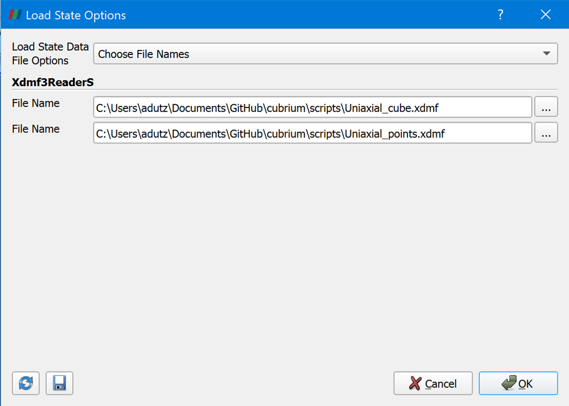
Import scene in ParaView.

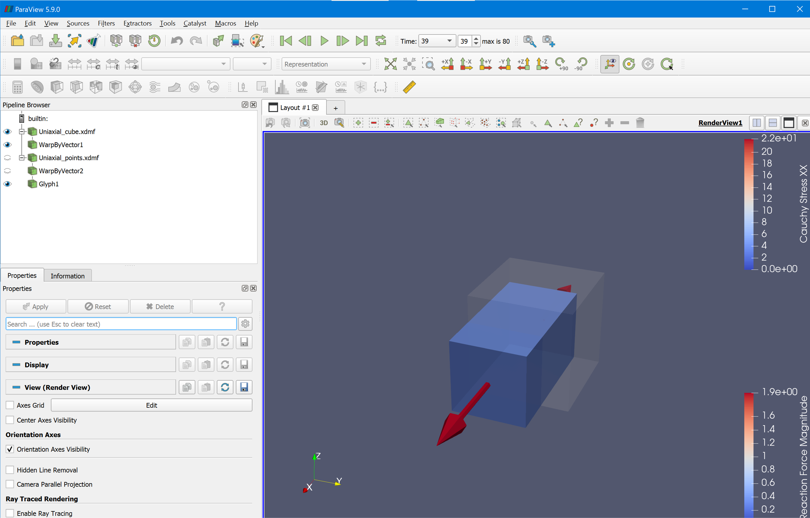
3D-view of the deformed cube with reaction forces in ParaView.

Animation of the cube-deformation in ParaView.

Have fun using cubrium! Please submit an issue if you find any bugs .